Optimizing speed and slope for stairclimbing using dynamic simulation
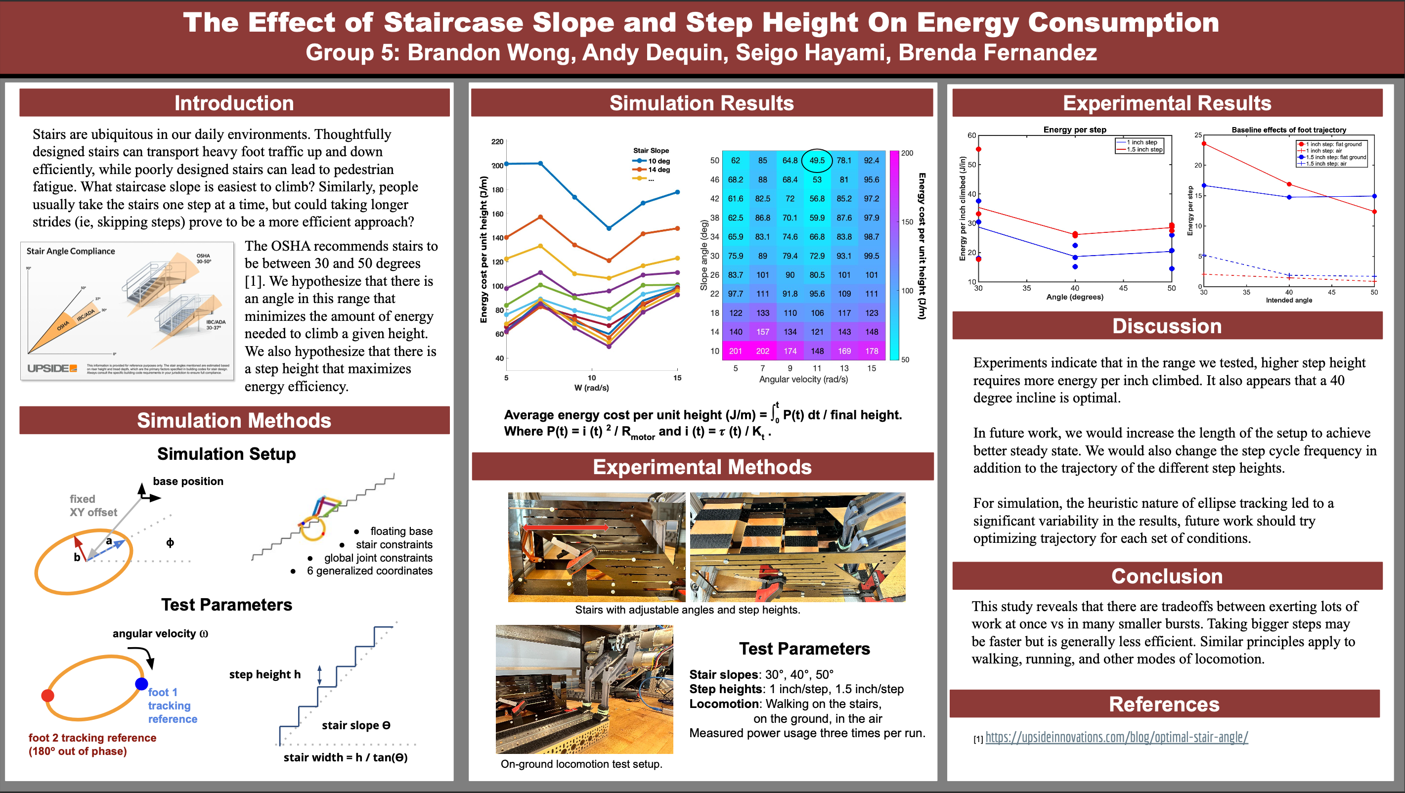
This page presents a summary of my final project for 2.74 Bio-inspired Robotics over Fall 2024.
The assignment is to find a phenomenon to study using a robotics hardware and dynamic simulation model. As a group of four, we decided to study the optimal speed to climb a set of stairs based on the slope.
My role was to implement a dynamics simulation and find estimated results. The simulation was manually and fully implemented in MATLAB for educational purposes, including Euler-Lagrange derviation of equations of motion, semi-implicit euler integration, impedance control with feedforward in cartesian coordinates, impulse-based constraints, and heuristic motion planning (ellipse tracking).

Simulation Setup
Since we are using 3D printed segmented legs from our lab, we started with code that defined each linkage's mass, position, and center of mass. In this setup code, the generalized coordinates of the simulation are defined, one for each motor and two for the position of the base in x and y. Then, the Euler-Lagrangian framework is used to derive the equations of motions for each generalized coordinate. The important information is then stored in helper functions for reference in the dynamic simulation script.
Defined Constraints
Once the simulation is setup, constraints need to be added to make the behavior more realistic.
- Staircase constraint: this represents the top of stair steps for given parameters. Implemented with impulse response.
- Joint constraints: this restricts the range of motion of the joints. Implemented with impulse response as well.
- Global angle constraints: emulating the gantry used in hardware which keeps the robot upright in the global frame. The joint constraint includes this as well.
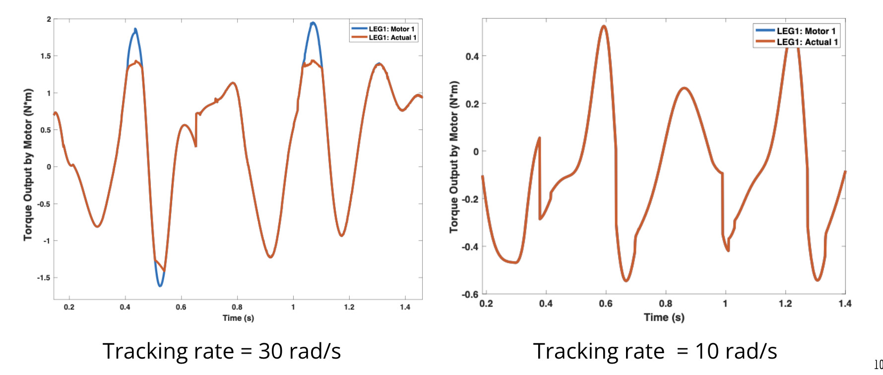
- Motor constraints: this represents the dynamics of an electric motor, limiting the possible power output to match the torque speed curve.

Controls
To simulate control, we opted to use a heuristic elliptical tracking method instead of a gradient-based optimizer for the sake of time. We did get practice using CasADi for trajectory optimization in a different exercise however. In the elliptical control scheme, we manually tune a set of ellipse parameters that define a trajectory for the robot's feet to follow. The only parameter that varies with the staircase parameters is the ellipse's slope. Once the ellipse trajectory is defined, an impedance controller with virtual spring and damper is used to track the trajectory.
Energy Tracking and Results
To determine efficiency, we devise a simple energy metric in J/m. To find the total energy spent, we use the motor power output integrated over time. To find the cost per unit height achieved we divide the total energy by the total height achieved by the end of the simulation.
i(t) = 𝝉(t) / Kt
P(t) = i(t) 2 / Rmotor
e = ∫ P(t) dt
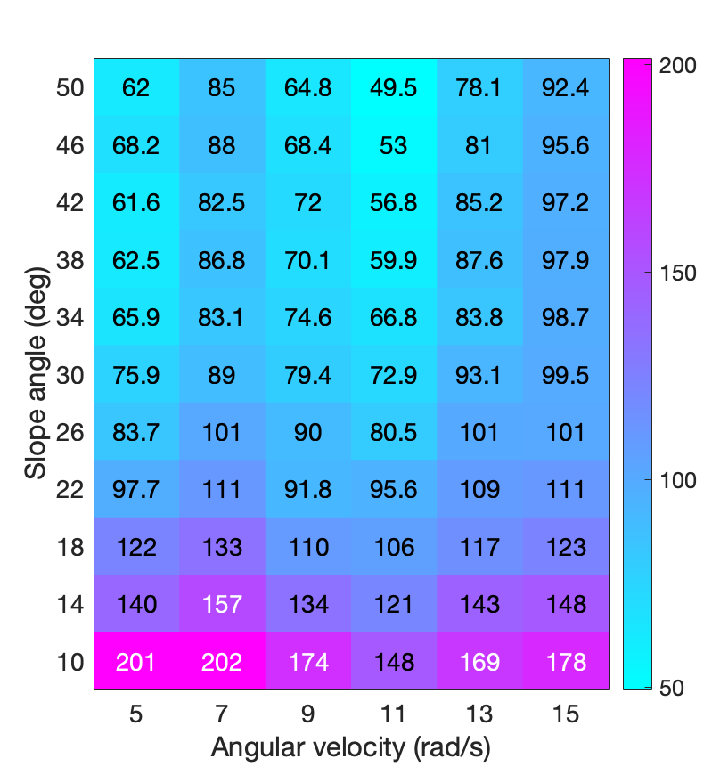
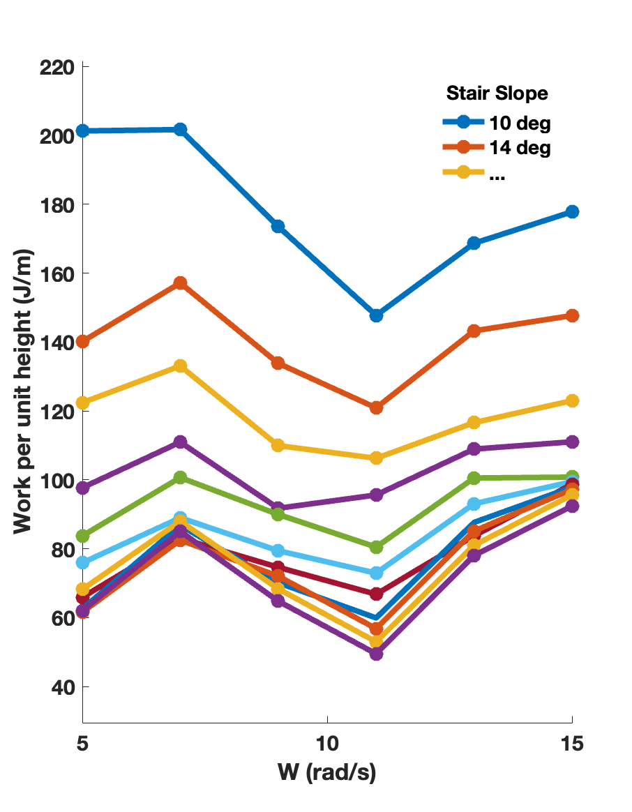
Once we have a metric with which to compare different performances, we sweep over the parameters we care about: How fast should we go depending on the slope? To answer this question, we sweep over the speed (ellipse tracking speed) and the slope (staircase angle).


From the simulation results, it appears that the optimal speed is around 11 rad/s at a 50 degree staircase angle. While the simulation may appear to show a consistent tradeoff, there are some caveats. It may have been useful to find the traveling speed by dividing the distance covered over time, as there are instances where tracking speed actually decreases effective traveling speed. The heuristic nature of the control scheme means that it was not truely optimal. In fact, it may be that the trajectory was optimized for steeper slope, and thus simulations with steeper slopes perfomed better. Some simulations ran into some failure cases due to low or high gain as well. Given the timeframe of four weeks to implement and run both simulation and hardware experiments, this was reasonable outcome, and certainly instructive. With more time however, there are many aspects that can be improved upon.